Here are slides and notes for a talk that was presented at AGU's 2018 fall meeting.
The context for this talk is that the State of California needs to know the spatial extent of aquifers that are fresher than 10,000 ppm TDS, particularly around oil fields so that it can regulate oil operators.
The California State Water Resources Control Board is working with the US Geological Survey on this problem, and I'm a sub sub contractor with the USGS, working on a less conventional approach, namely, using neural networks to map groundwater TDS with borehole geophysical logs as the input.
At this point, some of you are thinking: Why not just take measured TDS values from inside an oil field, and interpolate them into a map? It's because there isn't much measured TDS that's accessible to the public, at those depths. On the other hand, California oil operators have to file a borehole log with the State every time they drill, so the public has access to hundreds of thousands of these well logs, so it makes sense to try to derive TDS from that.
We've constructed a model that is used in the following way.
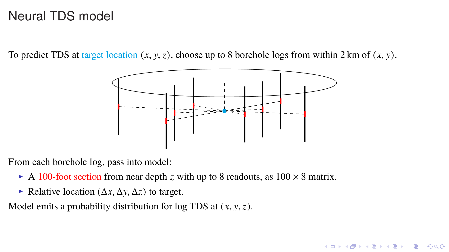
First pick a target point where a TDS prediction is desired.
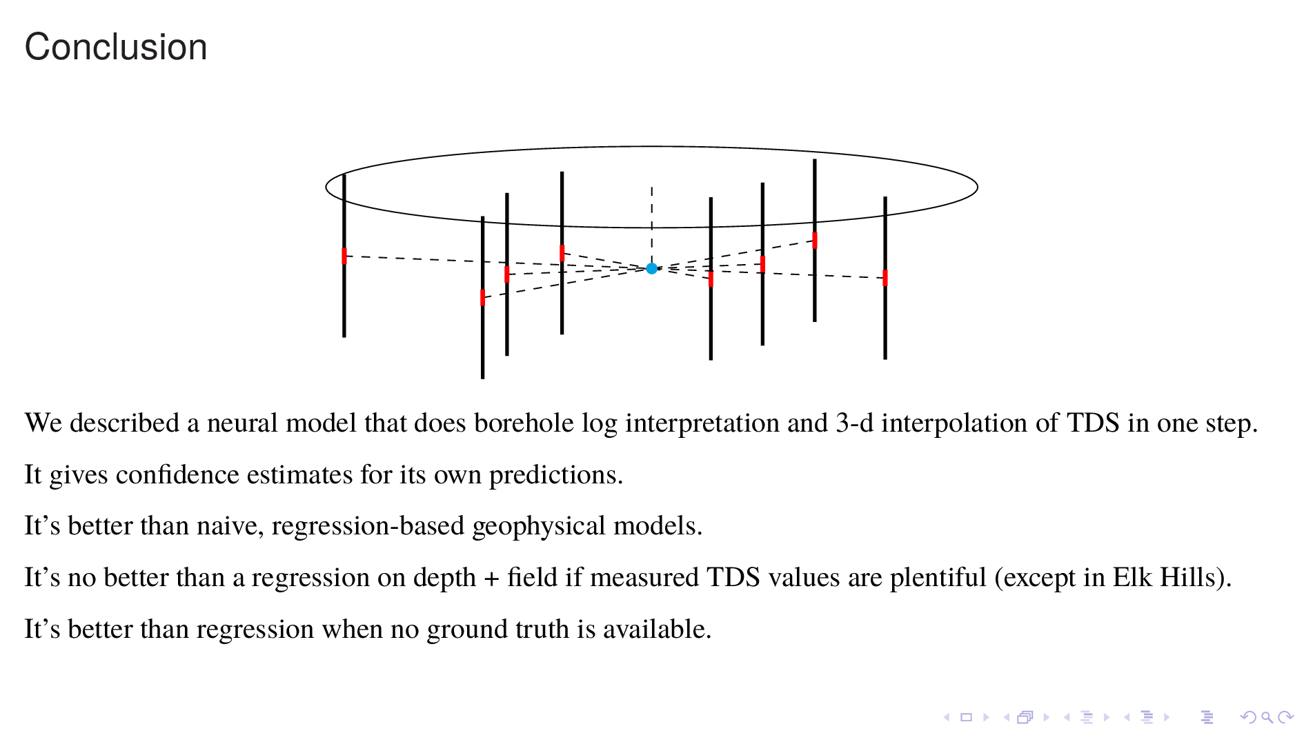
Then pick up to 8 borehole logs from within a 2 km radius of the target that overlaps the target in depth, and take a 100 foot section from each borehole log, with up to 8 readouts, and pass it into the model.
Also pass in the relative location of the borehole log section. The model does not need absolute locations, so that is not passed in.
The model outputs a probability distribution for the log of TDS at the target. This model essentially does borehole log interpretation and spatial interpolation, all in one step.
To build a volume map, we do this query for every point in the volume of interest.
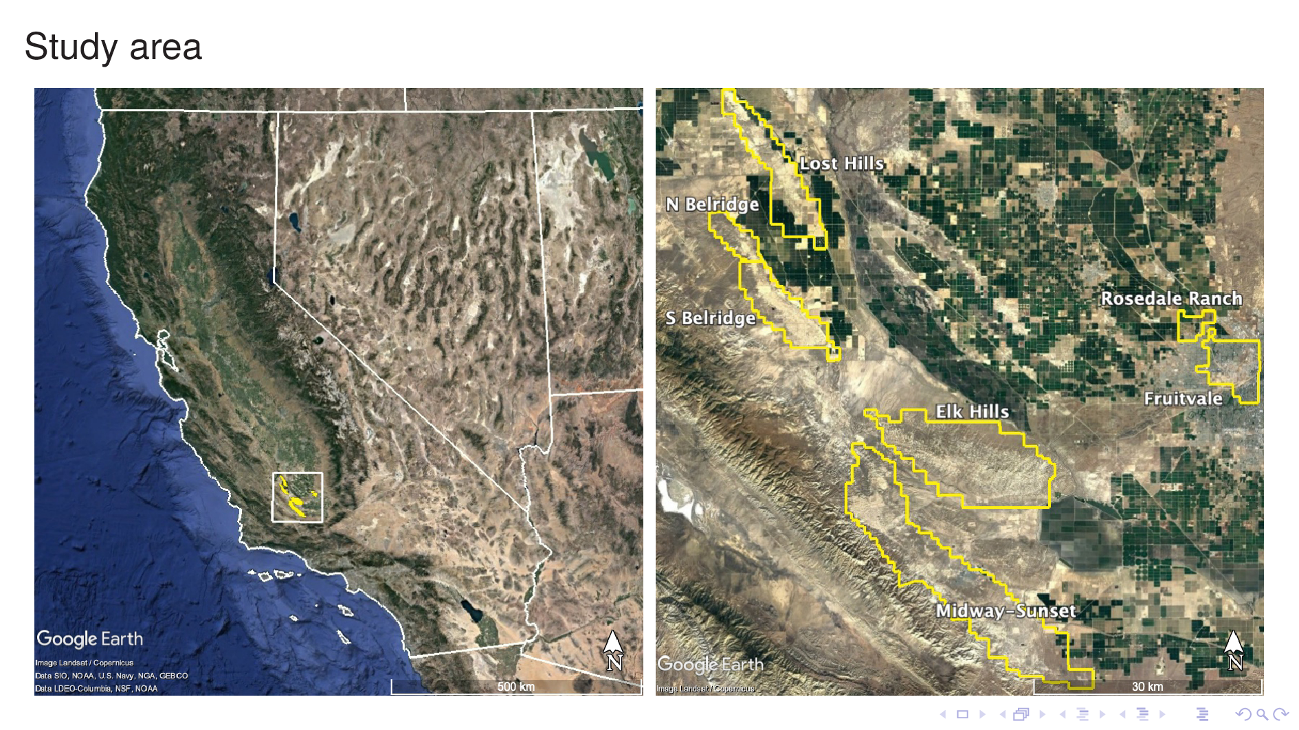
We developed this model by training it with data from seven Kern County oil fields, shown here. They lie at the rim of the southern tip of the Central Valley.
Our dataset consists of borehole logs and measured TDS values from each of these oil fields. Now I'll spend some time discussing this dataset.
Here I've shifted the oil fields around to make them fit on the screen, but their relative sizes are correct.
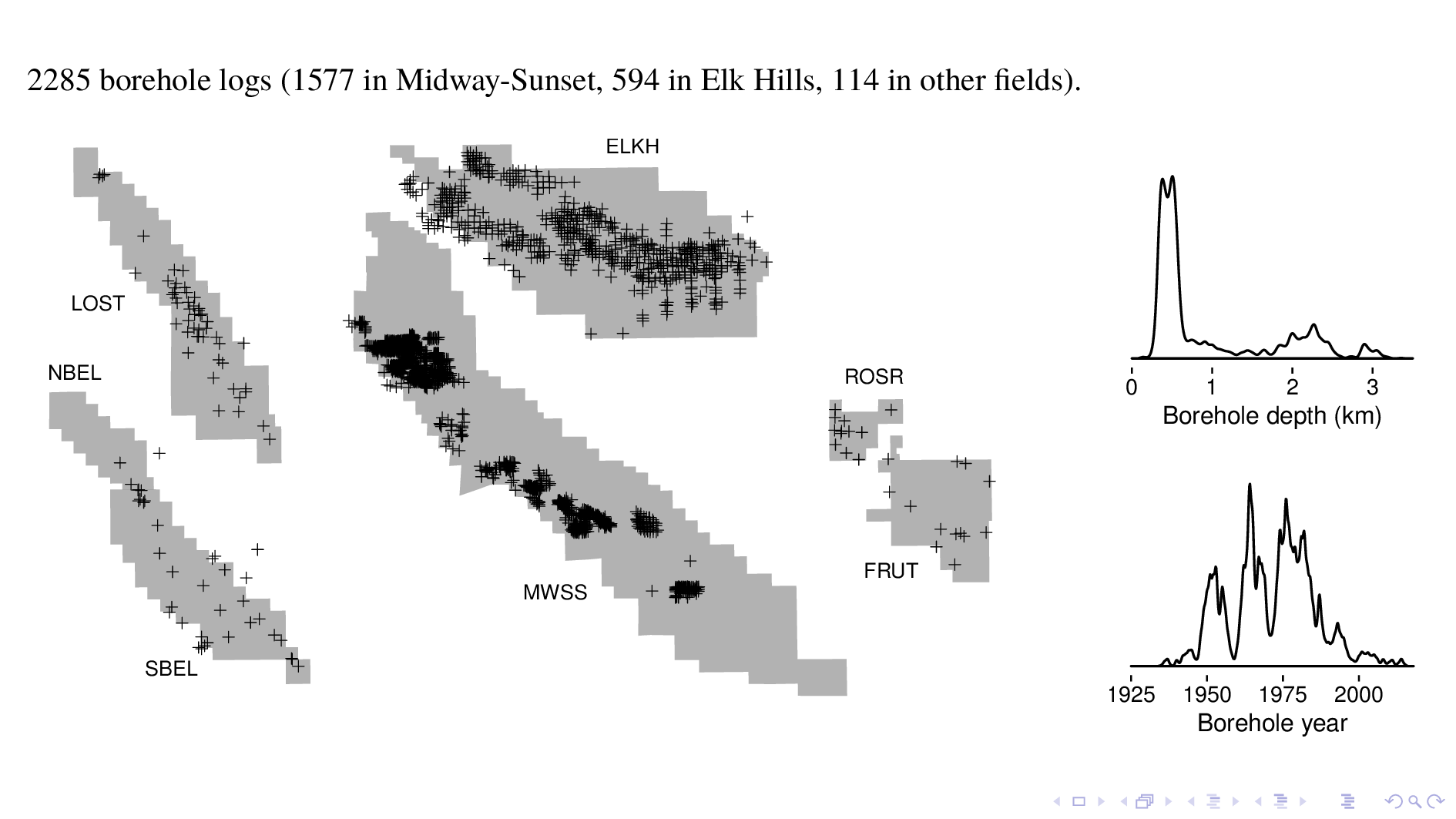
The model was trained with over 2000 borehole logs. Most are from a digital data dump we got from Chevron for MWSS, and another big chunk is from the Navy, which used to operate Elk Hills. We took care to discard borehole logs taken within 500 m of previous steam injection events, which disturbs geothermal gradients and make log interpretation difficult.
As you can see from the histogram of depth, many logs are as deep as 2 or 3 kilometers. As you can see from the histogram of time, most logs were taken in the 5 decades starting 1950.
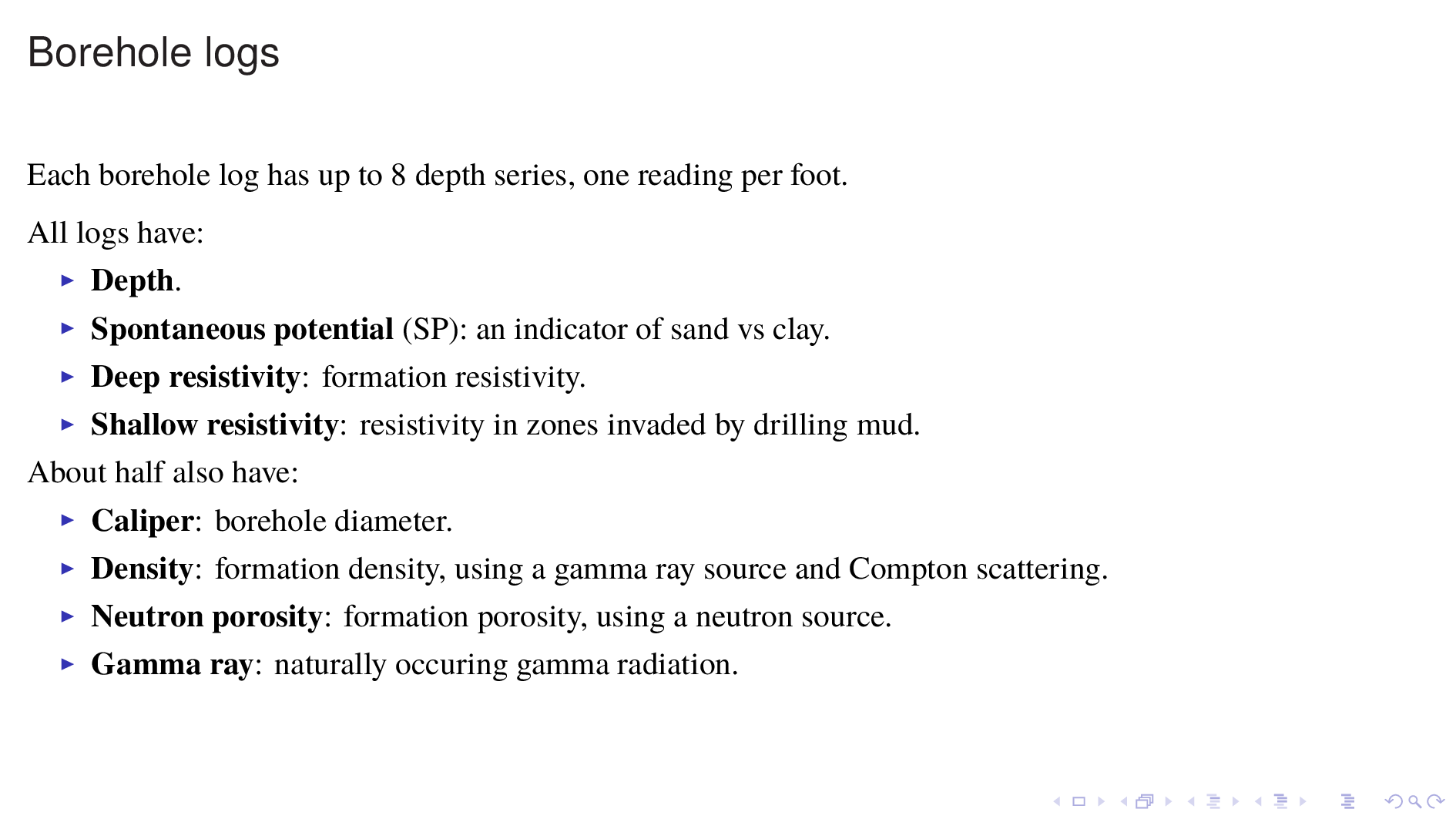
Borehole logs have up eight readouts, or depth series, with one reading per foot.
All of the logs have depth; spontaneous potential (which is an indicator of sand vs clay); deep resistivity, which gives formation resistivity; and shallow resistivity, which is the resistivity of zones invaded by drilling mud.
About half of the logs also have caliper readings, which gives borehole diameter; a density log, which gives formation density; a neutron log to indicate formation porosity; and a gamma ray log for naturally occurring gamma radiation.
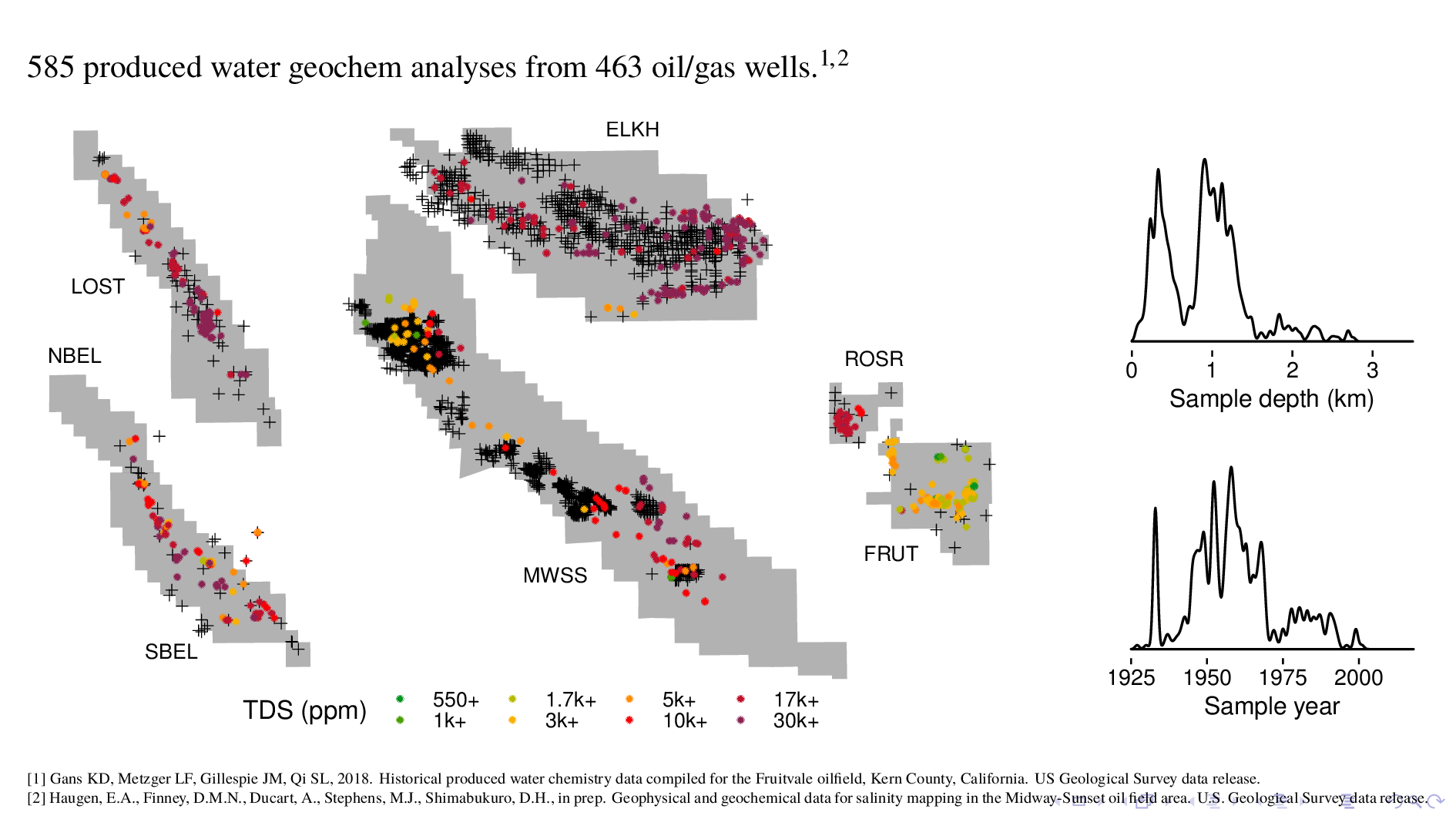
Now this is the other part of the dataset, which is geochem analyses that we use as ground truth for our model. These geochem are from produced water, which is the term of art for the waste fluid that comes up with oil during extraction. We're using around 600 data points, from roughly the same depths and times as the borehole logs.
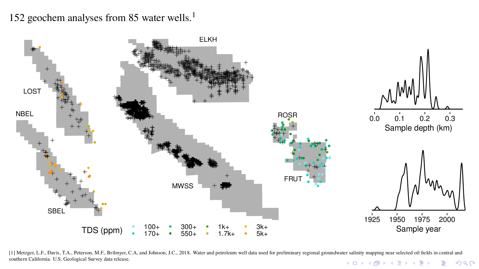
A second source of ground truth is water well geochem, which we have for some fields but not others. This data is useful because it's from a depth that is much shallower than produced water geochem.
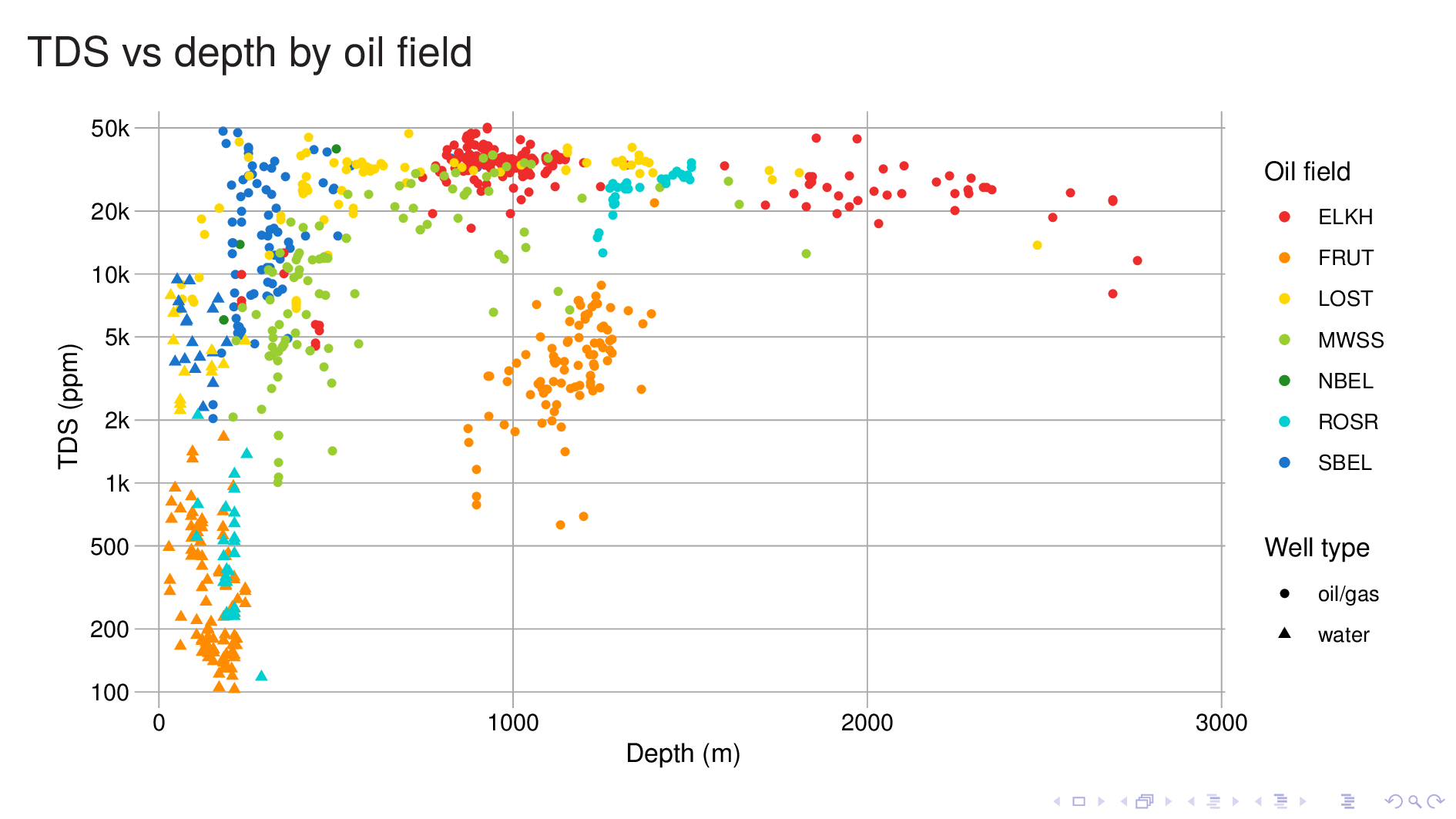
Here I plot TDS vs depth for all the geochem, and color it by the oil field, so we can get an idea of what we're dealing with. Two things jump out.
First, for any given field, depth is a good predictor of TDS. It turns out that a TDS model with just field and depth as input is actually quite good.
Second, the TDS/depth relationship varies a lot from field to field. If we look at the line where TDS is 10,000 ppm, we see that the depth at which an oil field reaches it varies from 200 m in the case of yellow (Lost Hills) to perhaps 1400 m for orange (Fruitvale). In fact our data for Fruitvale is all fresher than 10,000 ppm, and we have to extrapolate to get the answer.
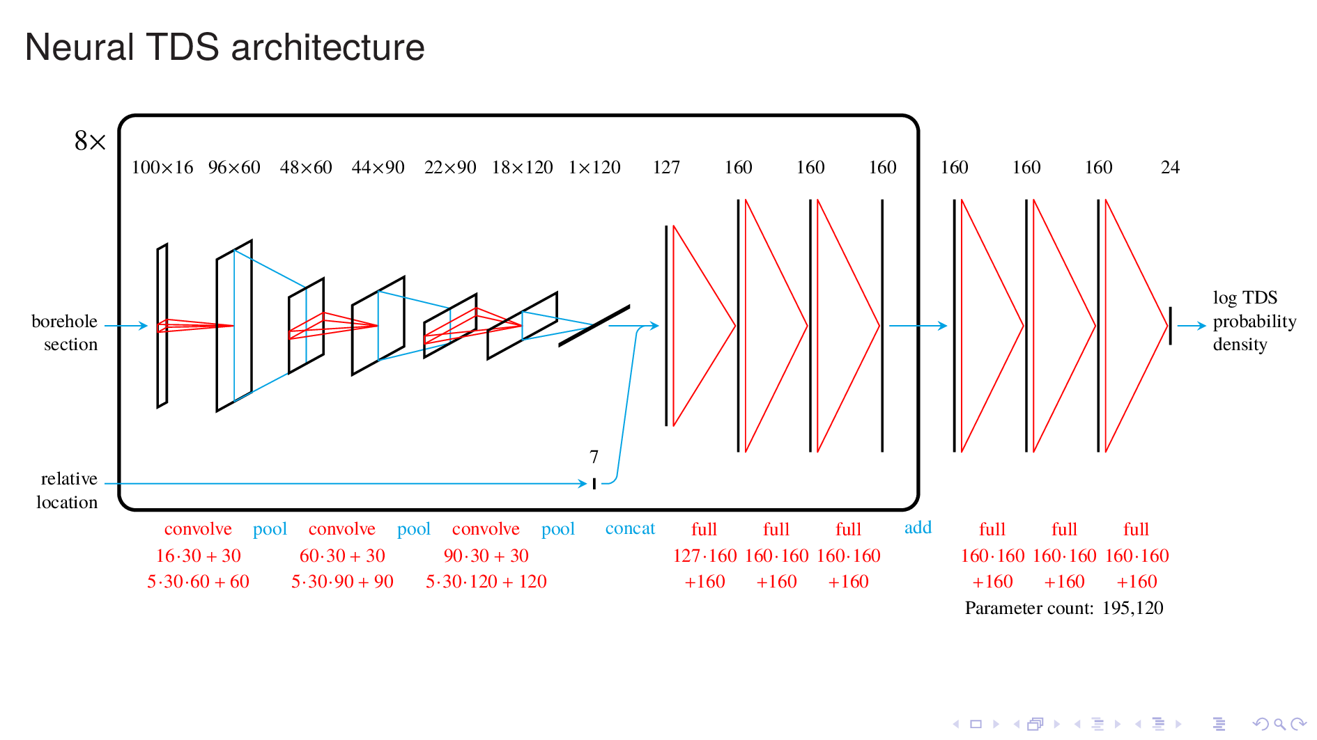
Under the hood, the neural TDS model looks like this.
The part inside the rectangular frame resembles a generic neural image classifer, which is the kind of model that takes for example, a picture of a cat, and tells you that it's a cat.
Borehole log interpretation resembles image classification in that it involves qualitative judgements, such determining lithology and fluid type.
Like an image classifier, this model takes a spatially correlated input and passes it thru many convolutional and pooling passes to press out meaningful features from the input. This is followed by fully-connected passes to produce an output.
In this model, there are eight of these units, running in parallel, one for each of the borehole logs. The outputs of these units are added together, and further processing gives a probability distribution for TDS at the target location.
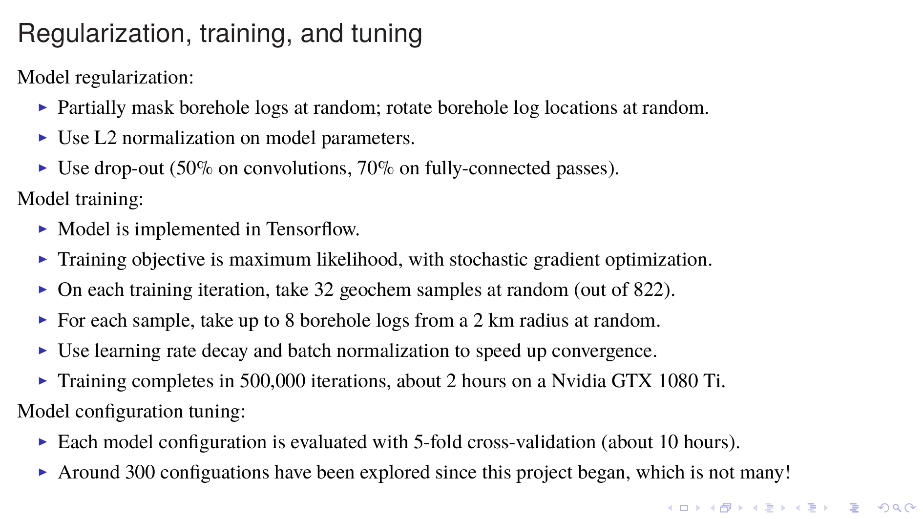
Here are details about how the model was regularized, trained, and tuned. This may be interesting only to other neural network researchers.
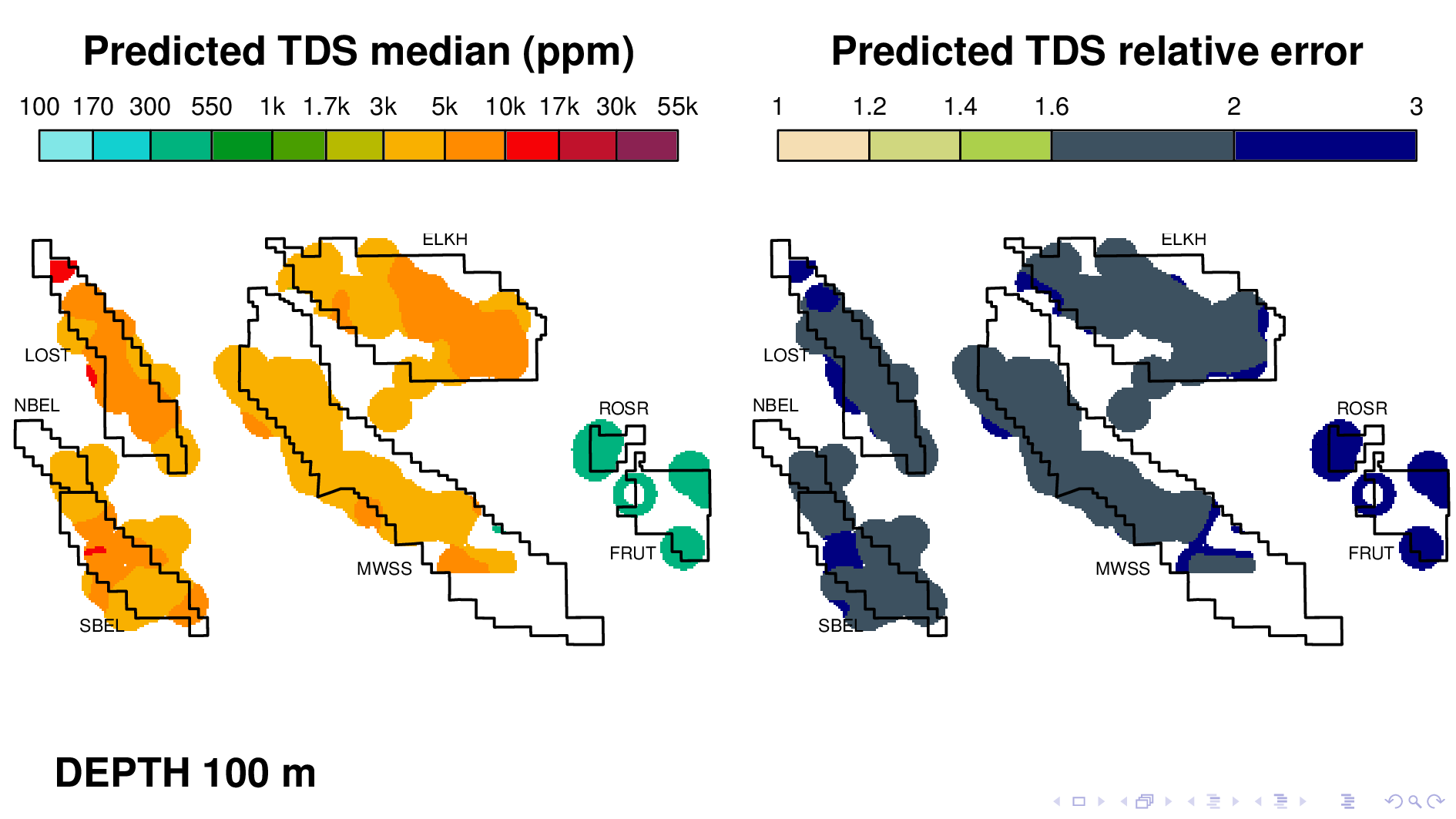
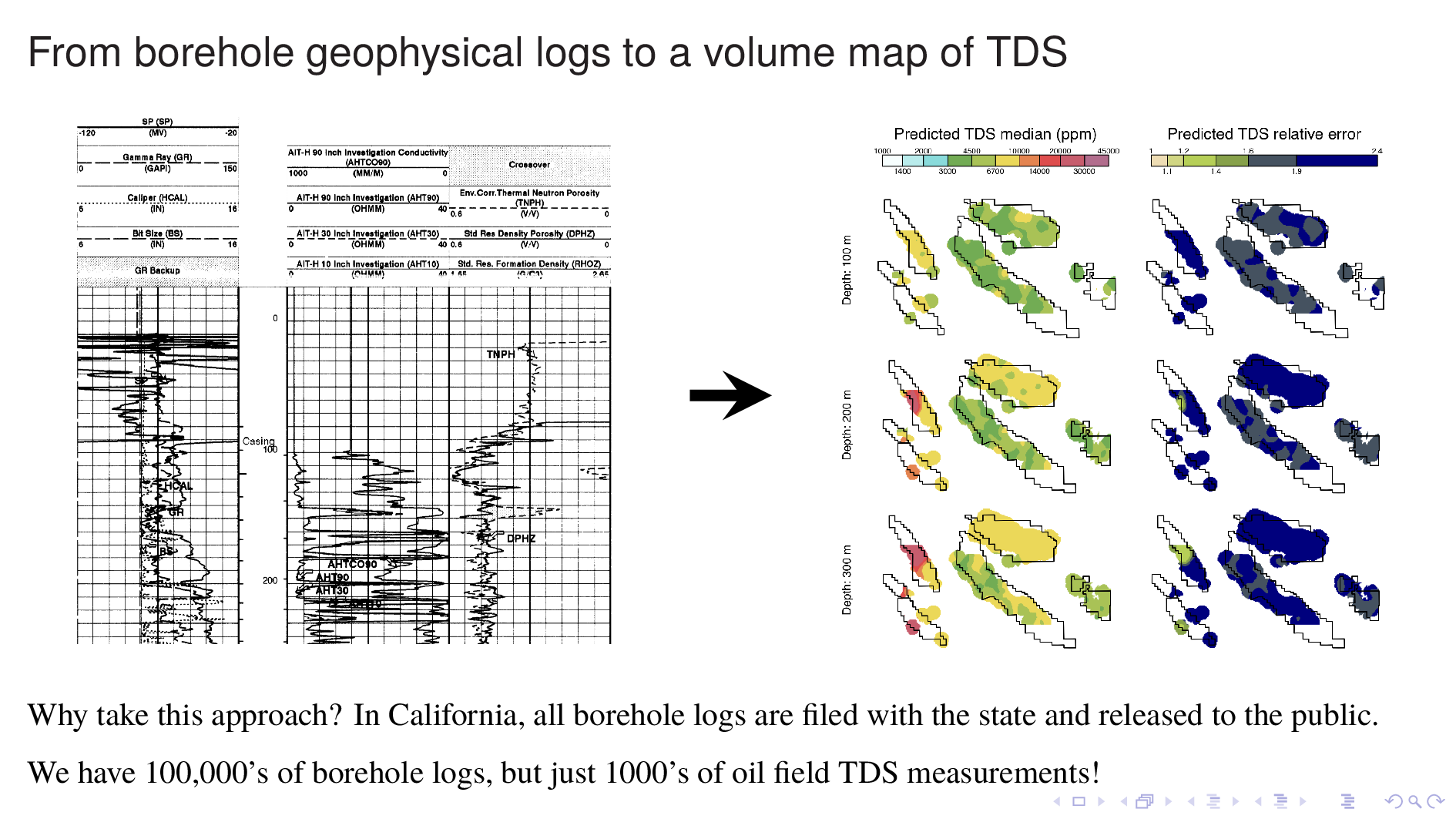
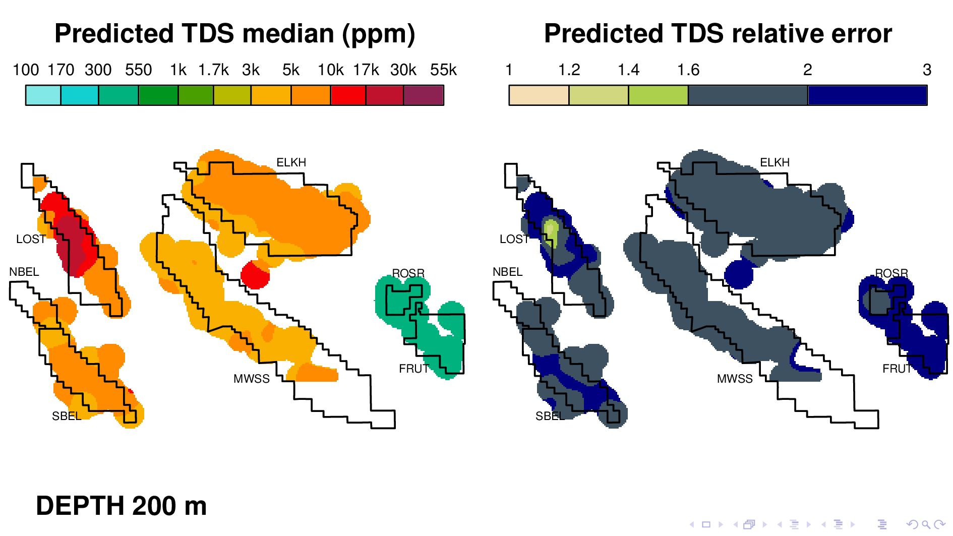
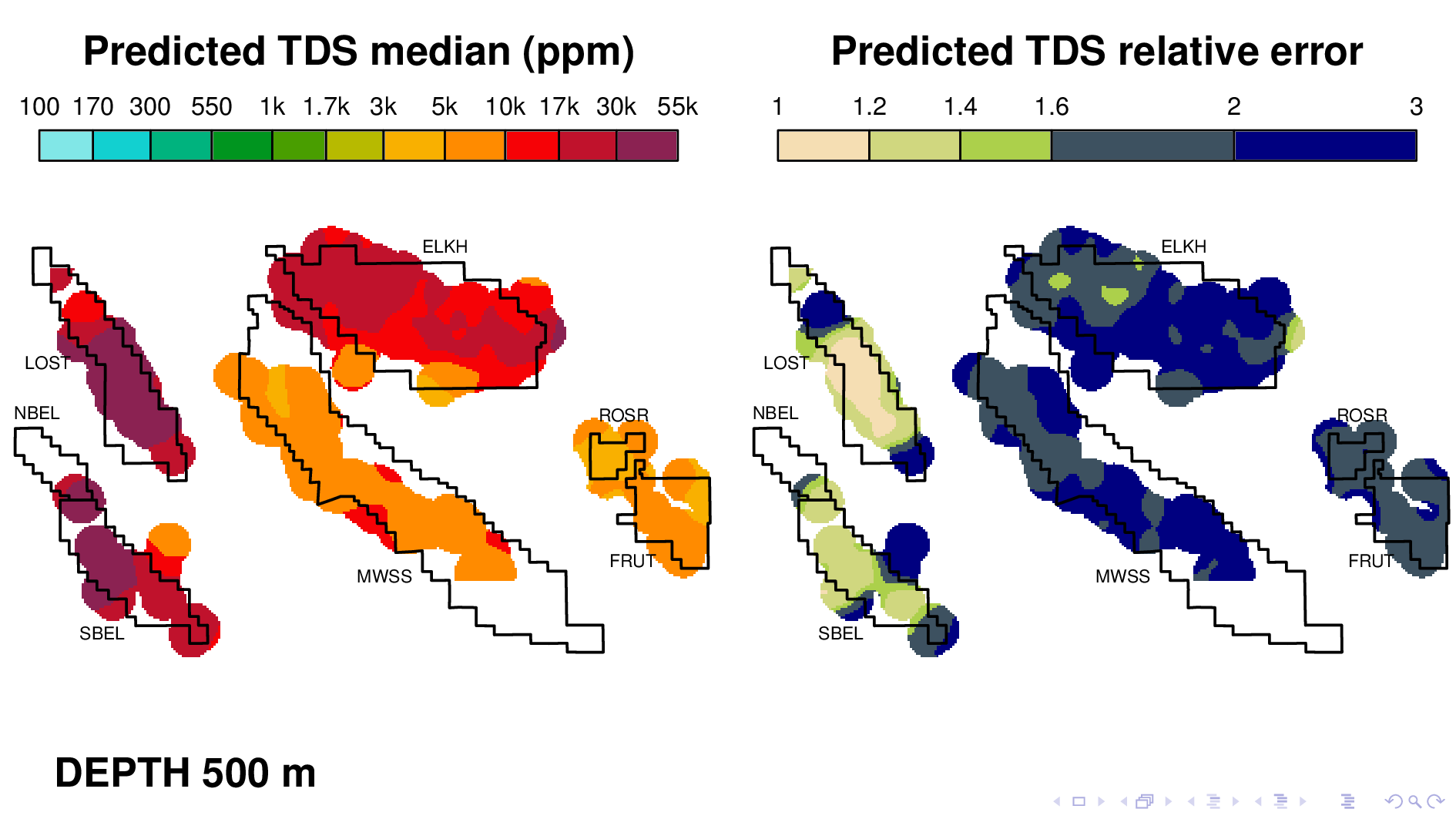
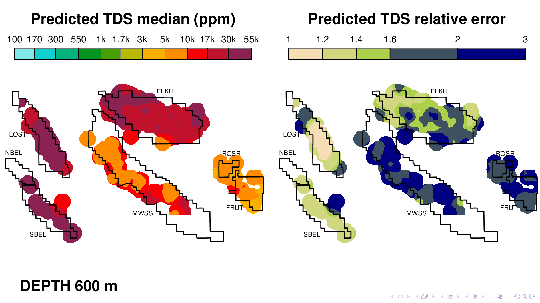
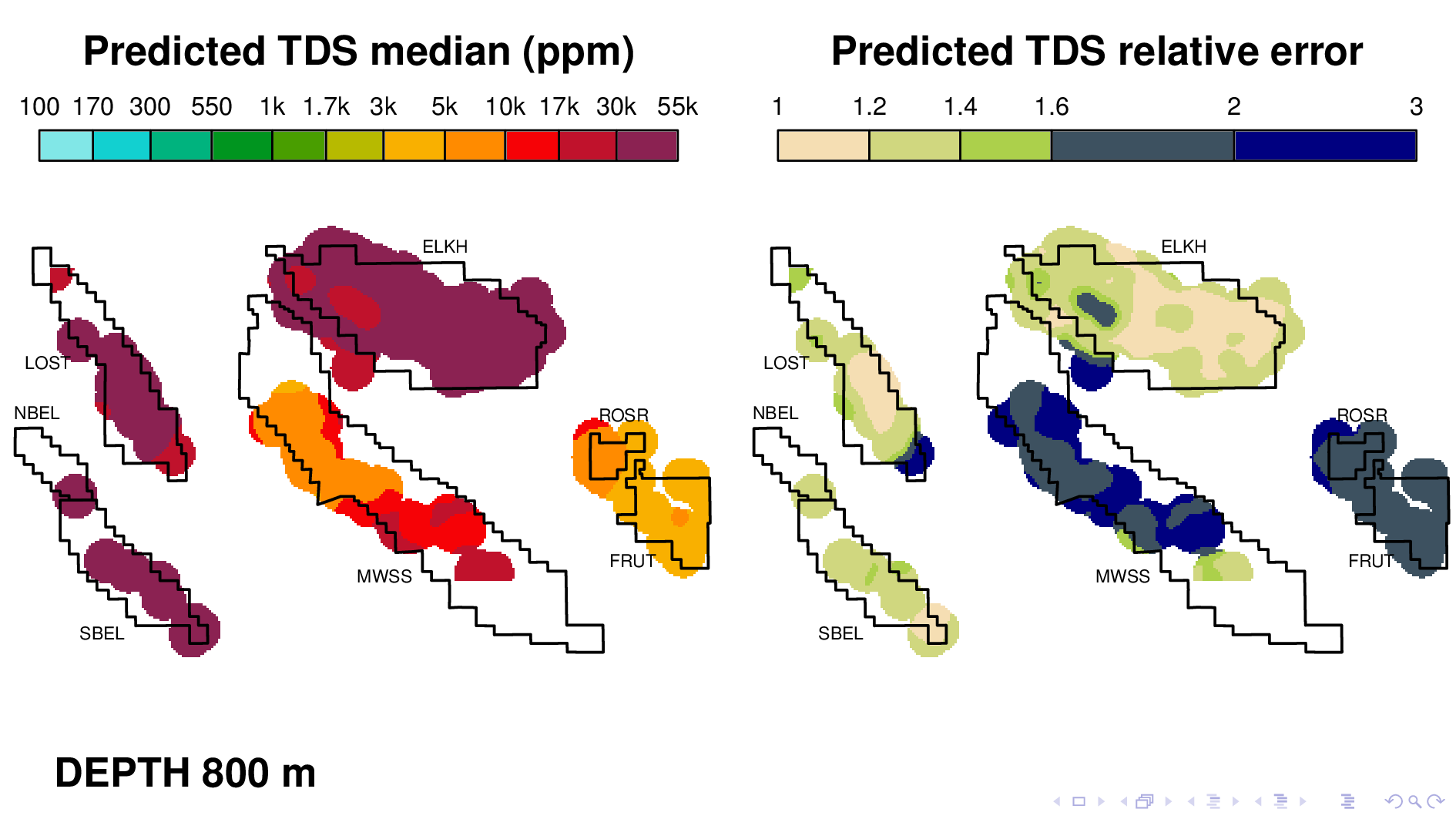
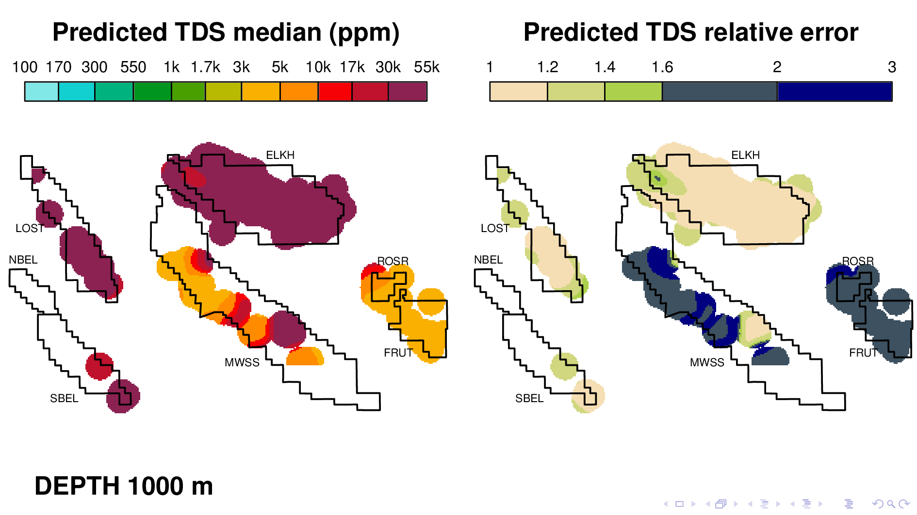
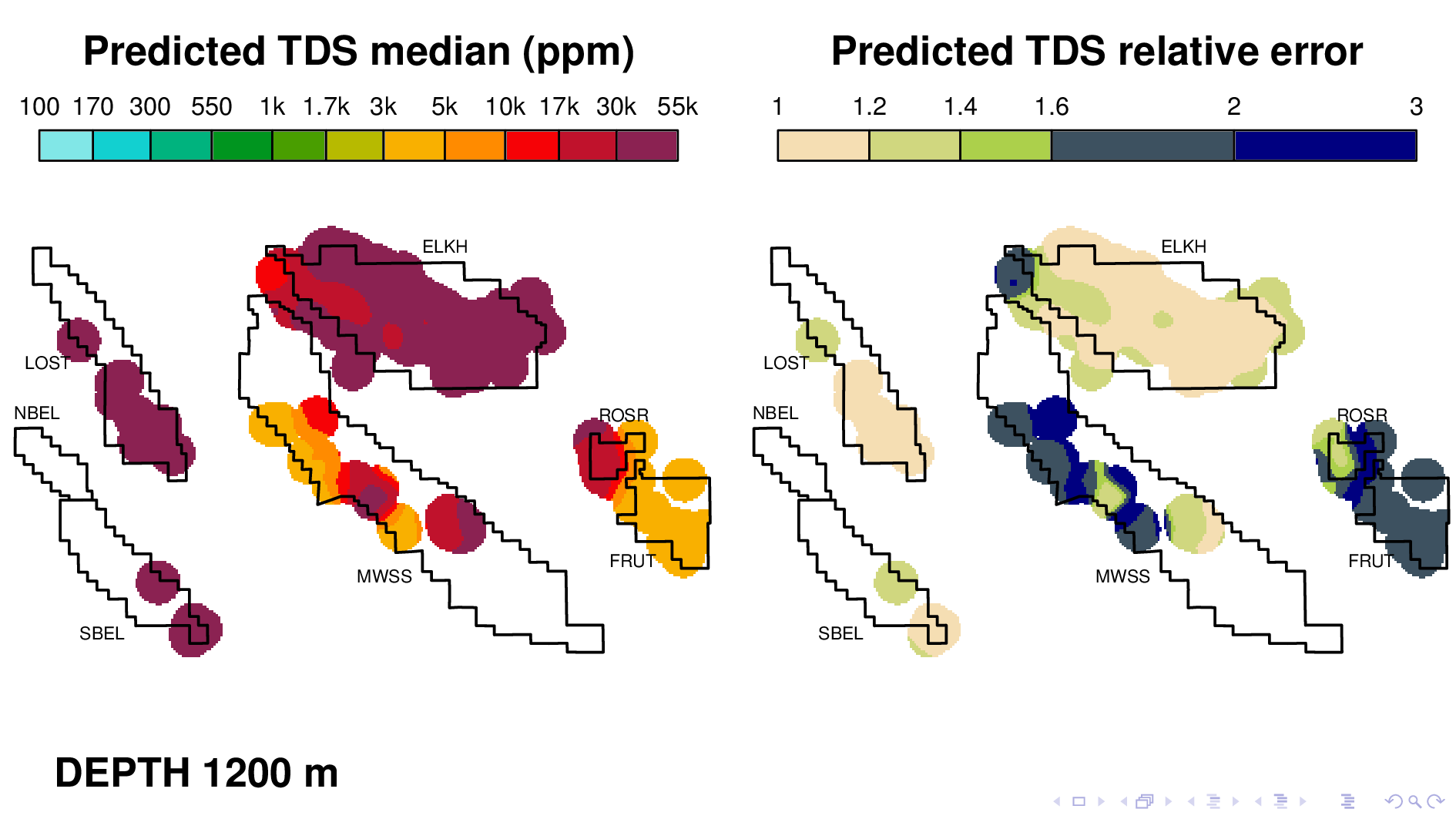
Here is the volume map produced by the neural TDS model. One the left is the predicted TDS median, in ppm. One the right is relative error, which indicates how confidant the model is in its own prediction. A relative error of 2, for example, means that most of the time, the truth is within a factor of 2 of what is predicted on the left.
Let me point out some things from these results. As expected, the model shows that each oil field transitions 10,000 ppm at different depths. (10,000 is red on this scale.) Now I'm going to flip though map views at different depths.
We see that Lost Hills transitions at 200 m,
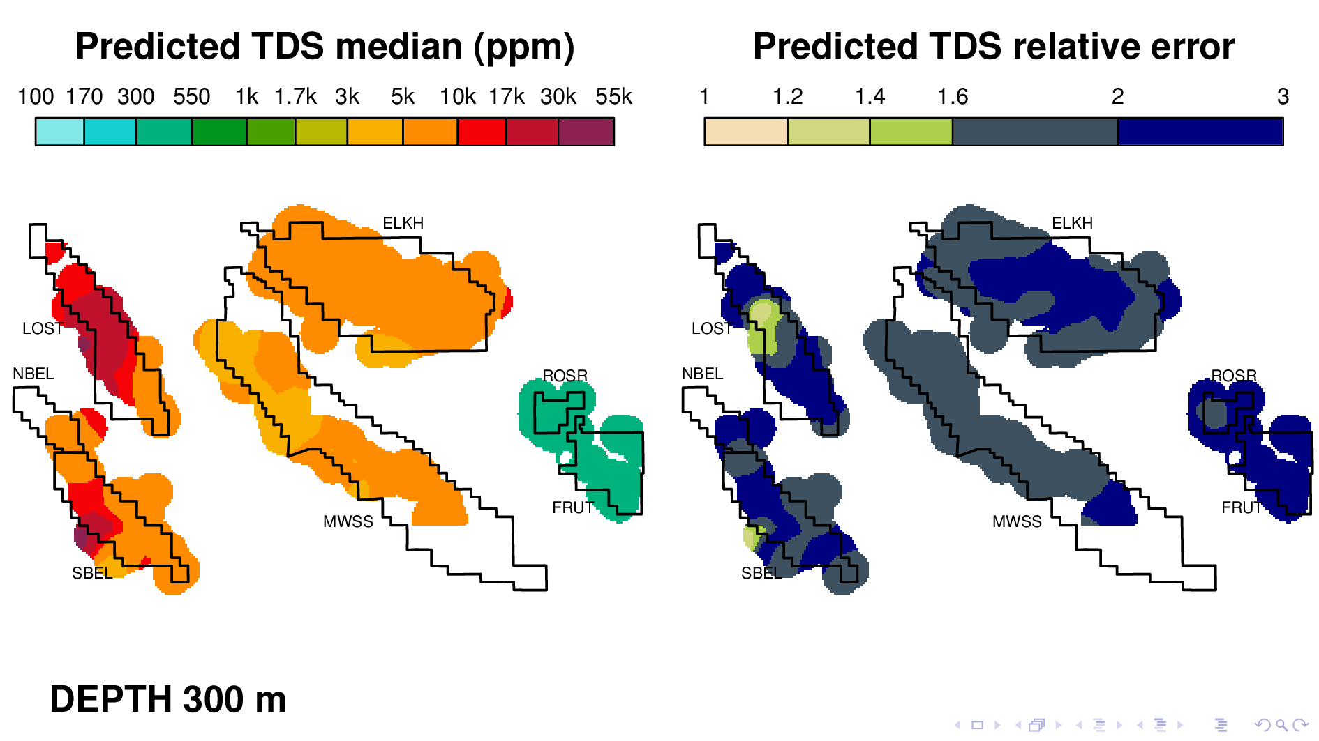
South Belridge at 300 m,
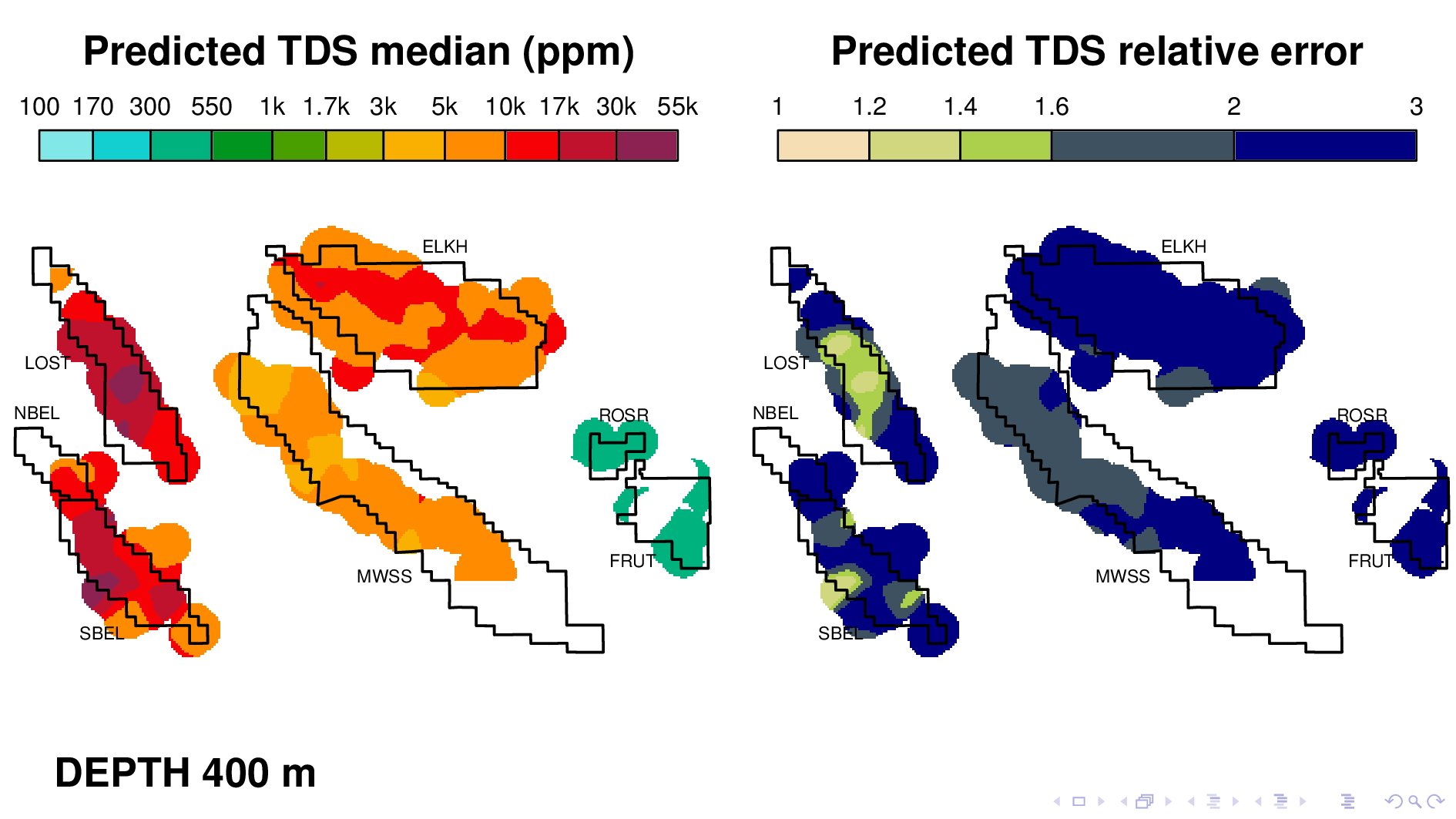
North Belridge and Elk Hills at 400 m,
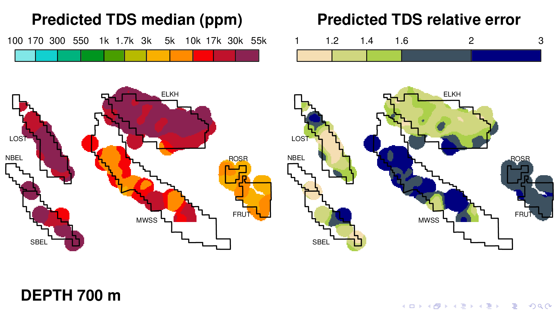
Midway Sunset at 700 maybe,
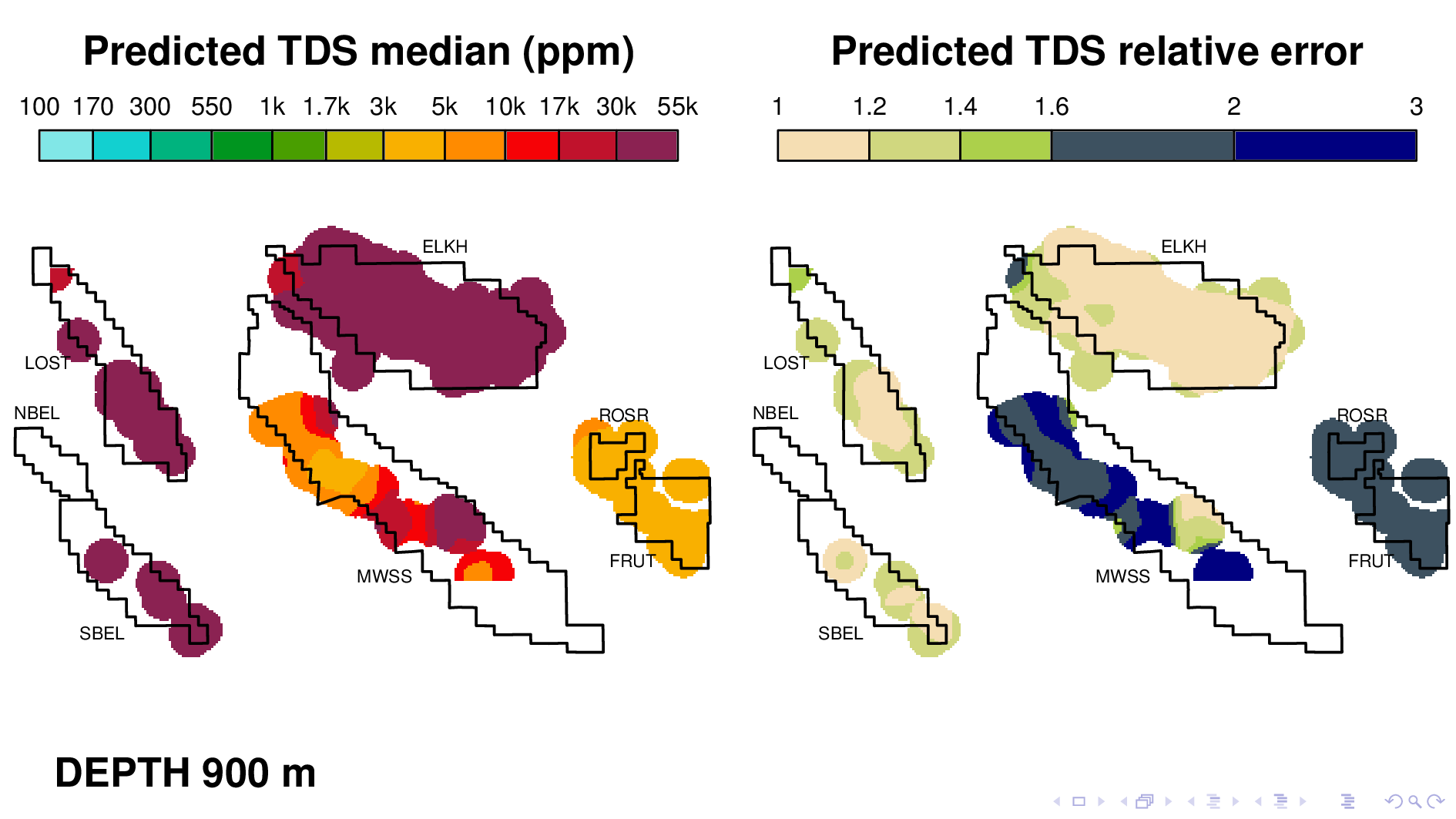
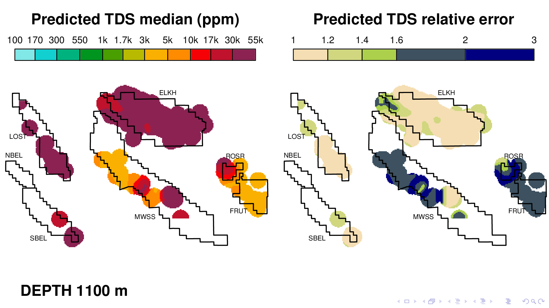
Rosedale Ranch at 1100,
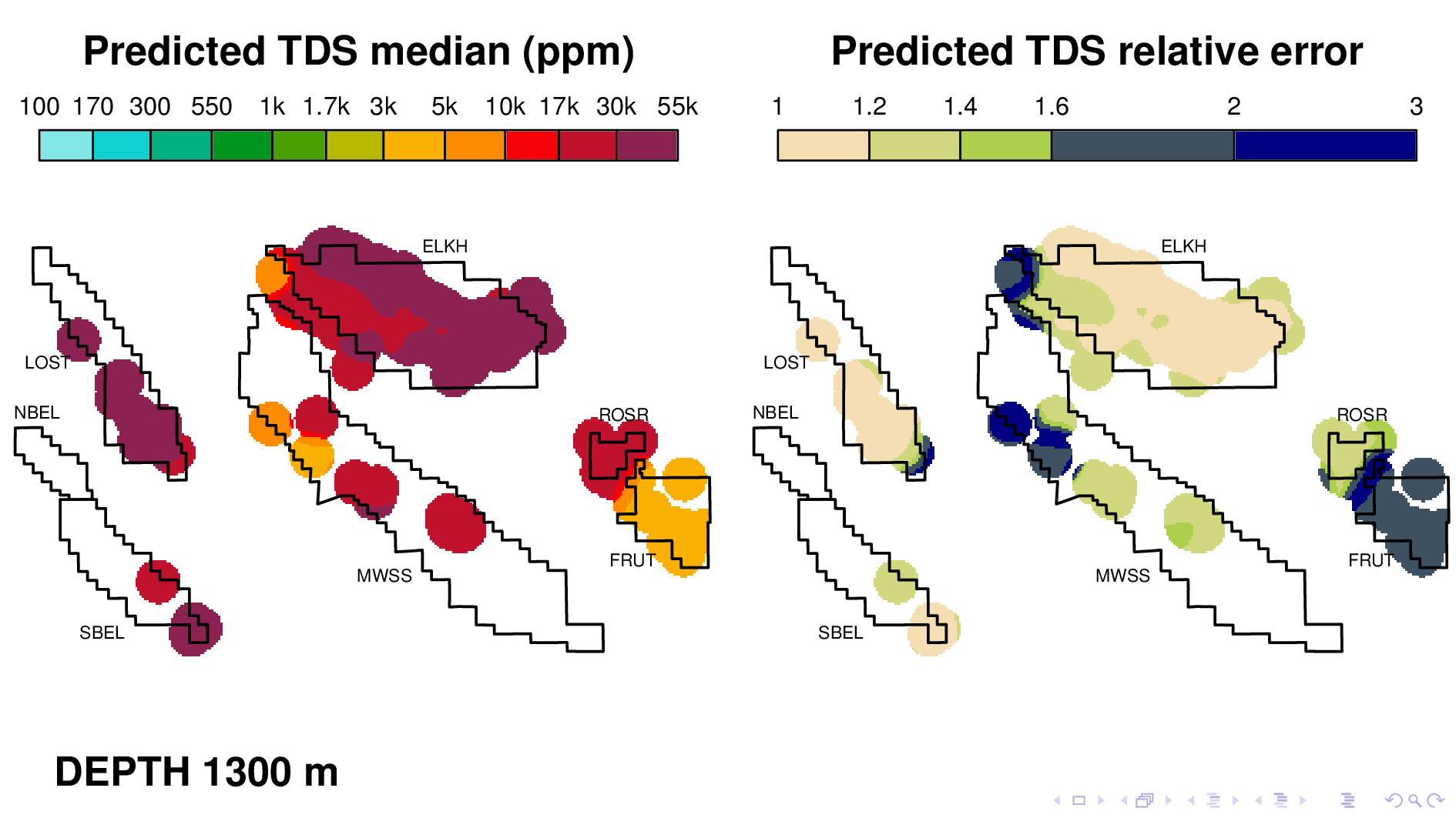
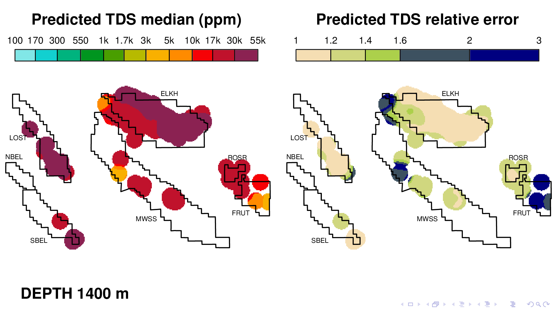
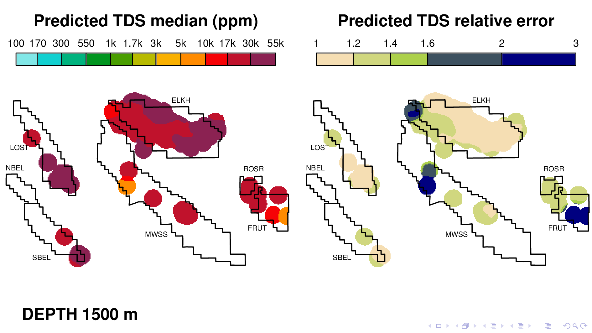
and Fruitvale at 1500. We know that the model is doing more than just recapitulating the data, because for Fruitvale, we lack ground truth TDS that exceeds 10000 ppm.

The model tends to be confident only when TDS values are as high as 30,000 ppm, perhaps because that's where most of its training data is. It's generally not very confidant when TDS is around 1000, which makes it less than ideal for its intended purpose. This slide shows Elk Hills reaching 10,000 ppm, but notice how large relative error is. This is something that we have to fix.

The model nonetheless captures some interesting phenomena, like for example this dramatic gradient in Rosedale Ranch at a depth of 1100 m. This gradient was first described by a coauthor in another paper that used traditional well log reading techniques. This is consistent with everything we know about this field, including the fact that a river runs right thru Fruitvale, which keeps the groundwater fresh going in that direction.
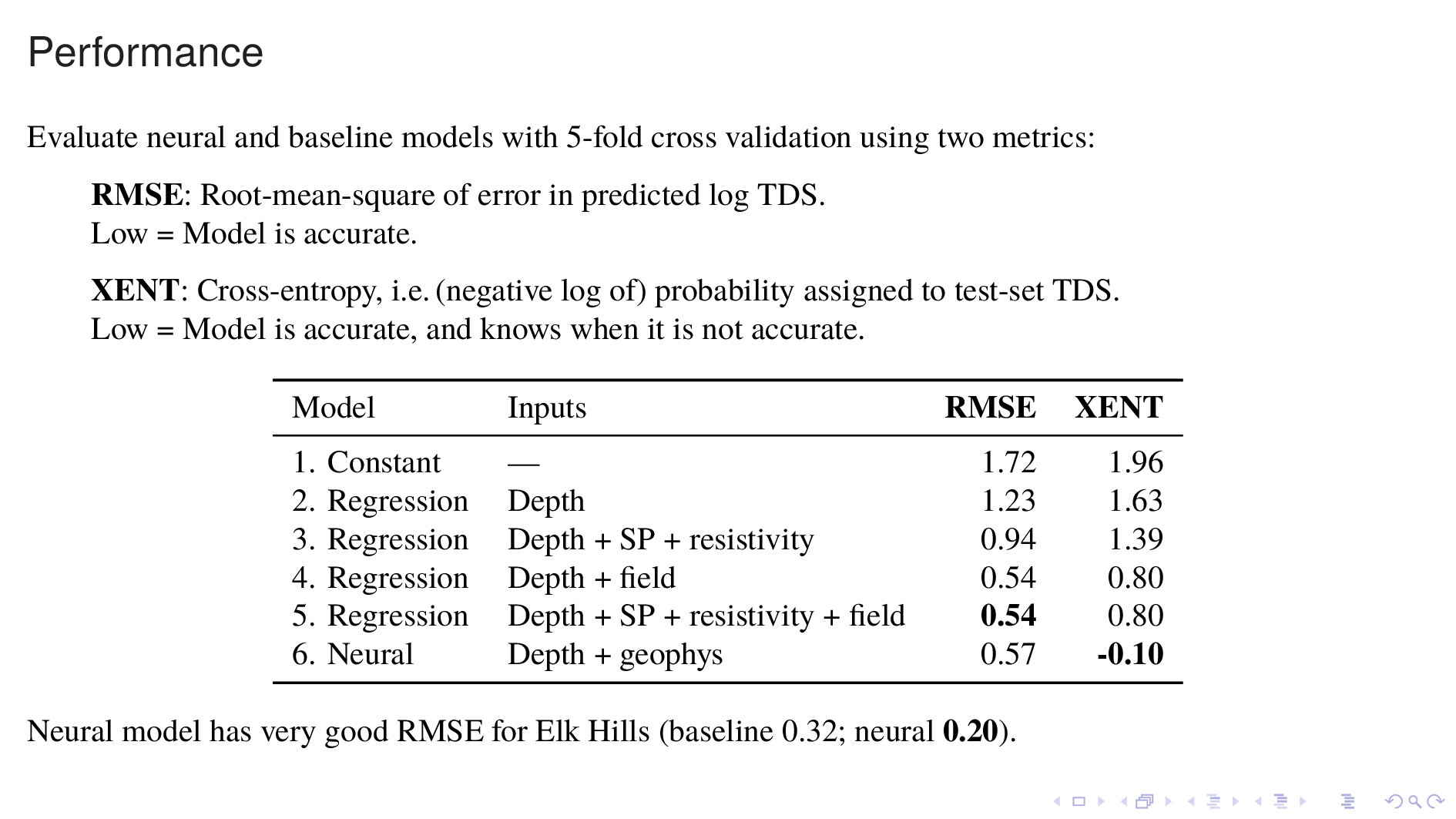
Now let's compare the neural model against various baseline models for predicting TDS.
I'll use two metrics: RMSE, or root-mean-square of error in predicted log TDS; and XENT, or cross-entropy, which is derived from the probability density that the model assigns to each TDS value in the test set. RMSE measures how much the model knows, whereas cross-entropy measures not just how much the model knows, but also how much it knows that it knows. For both metrics, lower is better.
Model 1 just guesses a constant for TDS everywhere. This does poorly, and simply gives an indication of the amount of variance in the data.
Model 2 is a polynomial regression on DEPTH. This also does poorly, because we know that different fields have very different TDS vs DEPTH relationships.
Model 3 incorporates statistics from some readouts from the nearest borehole log. This model constitutes a naive model for borehole log interpretation. It does substantially better, but is still quite bad.
Model 4 uses the identity of the field as an input, along with DEPTH and this model does very well, as expected.
Model 5 also incorporates information from the nearest borehole log, which improves it by a hair. This is the best baseline model and it's the one to beat.
Model 6 is the best version of the neural model that I have been able to construct so far. It actually does a bit worse than Model 5 in RMSE, which is a bit disappointing. But there are two bright spots.
One is that it does much better in cross-entropy. Cross-entropy is lower by about one, which means that it assigns about twice as much probability density to each TDS value in the test set. Another redeeming feature of the neural model is that it is far better than the baseline for one oil field in particular, which is Elk Hills. The reasons for this are unclear to me, but apparently borehole logs are very informative in this oil field.
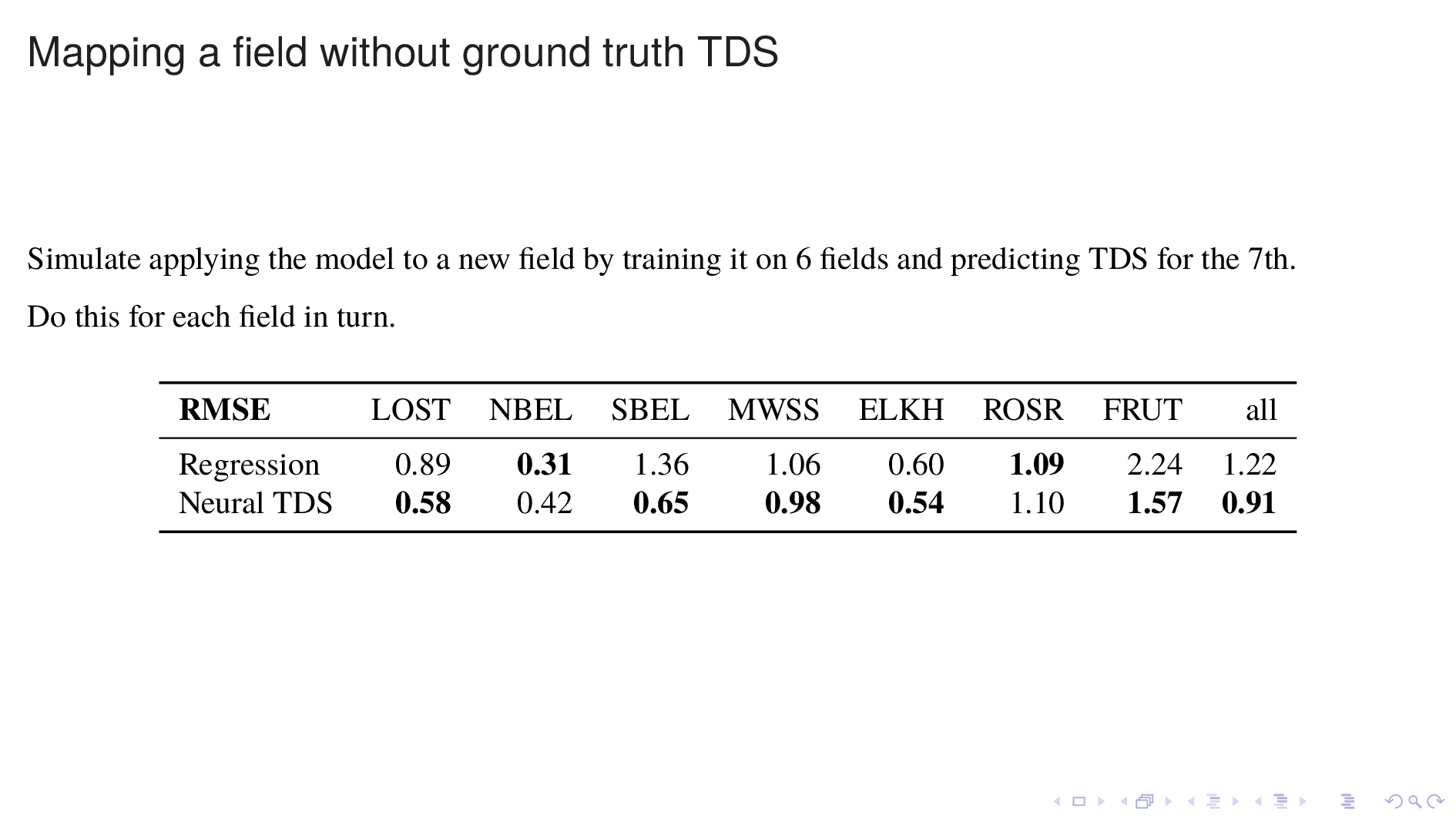
One way to improve the neural model would be to use the identity of the oil field as another input; but this doesn't play to the strengths of the model, which is location independent and field independent. Instead I decided instead to investigate how it would perform on a field that it has never seen before. After all, California has many oil fields where little or no ground truth data is available.
To simulate this condition, I train the model on 6 oil fields and use it to predict TDS values for the 7th. I do this for all 7 oil fields in turn, and I do the same with a regression-based baseline model.
This time, the neural model beats the baseline easily, judging by the aggregate score on the right. In Fruitvale, which is the most outlying in having the freshest water, the neural model is a big improvement. In other oil fields the neural model is usually better, and never much worse.